Handout week 49
AP Stats course Teacher: Hans van der Zwan Handout week 49
Literature Starnes D. S., et al. (2015). The Practice of Statistics (5th ed.). New York: W. H. Freeman and Company/BFW.
Handout per lesson
Lesson 1 Sun 2022-12-04
Theory
Topic: Transforming Random Variables Book: pp. 363-368
Preparation for lesson
See homework previous lesson
Class Activities
Discuss
Linear Transformations applied on Random Variables Influence of linear transformations on the Expected Value and Standard Deviation of a Random Variable are given by rules (1) and (2) below.
Note: rules (1) to (5) are given without a formal proof. The text book discusses most the rules using one example. Of course one example is not a formal proof!
Rule 1 If X is a random variable and Y = X + c (c a constant), then: \(\mu_Y=\mu_X+c\) and \(\sigma_Y=\sigma_X\) and \(VAR_Y~=~VAR_X\)
Rule 2 If X is a random variable and Y = cX (c a constant), then: \(\mu_Y= c \times \mu_X\) and \(\sigma_Y= |c| \times \sigma_X\) and \(VAR_Y~=~c^2~\times~VAR_X\)
Rule 3: combining rule 1 and rule 2 If X is a random variable and Y = a + bX (a and b constants), in other words Y is constructed by applying a linear transformation to X, then: \(\mu_Y= a + b \times\mu_X\) and \(\sigma_Y= |b| \times\sigma_X\) and \(VAR_Y~=~b^2~\times~VAR_X\)
Example The relationship between temperature in \(^0F\) and \(^0C\) is: \(Temperatuur~in~^0F~=~32~+~\frac{9}{5}\times~Temperature~in~^0C\)
Define the random variable T: the maximum temperature in Amman on a randomly chosen day in October in degrees Celsius. Based on historical data, \(\mu_T = 28.6^0C\) and \(\sigma_T = 4.0^0C\). The random variable F is defined as the maximum temperature in Amman on a randomly chosen day in October in degrees Fahrenheit. The question is, what are \(\mu_F\) and \(\sigma_F\)? Applying rule 3: \(\mu_F~=~32~+\frac{9}{5}~\times~\mu_X~=~32~+\frac{9}{5}~\times~28.6~=~83.5~^0F\) \(\sigma_F~=~\frac{9}{5}~\times~\sigma_X~=~\frac{9}{5}~\times~4.0~=~7.2^0F\)
Figure 48.1 Maximum Daily Temperatures in October in Amman, 1979 to 2013
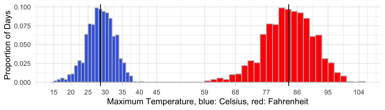
Note. The black lines indicate the mean in \(^o\)C resp. \(^o\)F. The mean in \(^o\)F is 83.5 which is \(\frac{9}{5}\) times the mean in \(^o\)C (28.6) + 32. The spread of the vales in \(^o\)F is a factor \(\frac{9}{5}\) higher than the spread of the values in \(^o\)C.
Exercises 6-39 and 6-40
Rules for Sum of Random Variables
Rule (4) If X and Y are two random variables and S = X + Y and D = X - Y then: 4a. \(\mu_S~=~\mu_X~+~\mu_Y~~~~~or~~~~~\mu_{X+Y}~=~\mu_X~+\mu_Y~~~~~or~~~~~E(X+Y)~=~E(X)~+~E(Y)\) 4b. \(\mu_D~=~\mu_X~-~\mu_Y~~~~~or~~~~~\mu_{X-Y}~=~\mu_X~-~\mu_Y~~~~~or~~~~~E(X-Y)~=~E(X)~-~E(Y)\)
Rule (5) (5) If X and Y are two independent random variables and S = X + Y then: \(VAR_S~=~VAR_X~+~VAR_Y~~~or~~~\sigma_{X+Y}^2~=~\sigma_X^2~+~\sigma_Y^2\)
this rule only applies for two independent random variables; be aware not to add up the standard deviations of X and Y, but the variances.
Exercise 6-47
From rule (4) follows rule (5):
- If X and Y are two independent random variables and D = X - Y then: \(VAR_D~=~VAR_X~+~VAR_Y~~~or~~~\sigma_{X-Y}^2~=~\sigma_X^2~+~\sigma_Y^2\)
Proof of rule (6) It is easy to understand that the Variance of the random variable W = -Y is equal to the Variance of the random variable Y after all they have the same spread; so: \(VAR_{(-Y)}~=~VAR_Y\) Now if V = X - Y then V = X + (-Y) and: \(VAR_V~=~VAR_X~+VAR_{(-Y)}~=~VAR_X~+VAR_Y\)
Exercise 6-57, 6-58
Distribution of the Sum and Difference of Normal Distributed Random Variables
Rule (7) (7a) If X and Y are Independent Random Variables, both with a Normal Distribution, and S = X + Y, then S has a Normal Distribution as well, with according to rule (4) \(\mu_S = \mu_X + \mu_Y\) and according to rule (5) \(\sigma_S^2~=~\sigma_X^2~+~\sigma_Y^2\)
(7b) If X and Y are Independent Random Variables, both with a Normal Distribution, and S = X - Y, then S has a Normal Distribution as well, with according to rule (4) \(\mu_S = \mu_X - \mu_Y\) and according to rule (6) \(\sigma_S^2~=~\sigma_X^2~+~\sigma_Y^2\)
Distribution of a Linear Transformed Normal Distribution Rule (8) (not in the text book) (8) If X is a Random Variable with a Normal Distribution and Y = a + bX, then the distribution of Y is Normal as well and according to rule (3) \(\mu_Y = a + b \times \mu_X\) and \(\sigma_Y = |b| \times \sigma_X\)
Exercise 6-61
Homework
Exercises 6-39 and 6-40
Homework to hand in
Lesson 2 Mon 2022-12-05
Learning Objectives
SKILL_ID | SKILL | TOPIC_ID | TOPIC | LO_ID | LEARNING_OBJECTIVE |
3B | Determine parameters for probability distributions. | 4.9 | Combining Random Variables | ||
3C | Describe probability distributions. | 4.9 | Combining Random Variables |
Preparation for lesson
See homework previous lesson
Theory
Topic: Combining Random Variables Book: pp. 369-379
Class Activities
Discuss
Application of the rules about combining and transforming random variables By filling processes, not every product will have exactly the same contents or weight. What is allowed and what not, is in many countries regulated by Law. See for instance UK regulations. The Three Packers Rules below come from this website.
Three Packers Rules These set out 3 rules that packers and importers must comply with:
- The contents of the packages must not be less on average than the nominal quantity
- The proportion of packages which are short of the stated quantity by more than a defined amount (the ‘tolerable negative error’) should be less than a specified level
- No package should be short by twice the tolerable negative error
They provide protection for consumers on short measure.
Generally the contents or the weights of packages are Normally Distributed. If the contents is said to be 1,000 gram, not every package has to contain at least 1,000 gram. A certain percentage that contains less is legally allowed. But, on average the contents must be 1,000 gram and there are rules for the proportion of packages that contain less than 1,000 gram.
Exercise and (fully) worked out answers on a gray background The weights of packages with sugar are approximately normally distributed with a mean of 1,000 gram and a standard deviation of 15 gram.
Let X be the contents of a randomly chosen package sugar X ~ N(1,000; 15) gram
- What proportion of the packages contain less than 980 gram?
P(X < 980) = 0.0912 (graphic calculator) or P(X < 980) = P(Z < \(\frac{980-1000}{15})\) = P(Z < -1.33) = 0.0918 (book table T-1) The proportion that contains less than 90 gram is 0.091 (of 0.092)
- What proportion of the packages contain between 980 and 1,020 gram?
P(980 < X < 1,020) = 0.8176 (graphic calculator) Proportion between 980 and 1,020 is 0.818
- What proportion of the packages contain between 970 and 1,010 gram?
P(970 < X < 1,010) = 0.7248 (graphic calculator) Proportion between 970 and 1,010 is 0.725
Someone buys three packages of sugar. Define Xi: the contents of the iˆth package.
- It is assumed that X1, X2 and X3 are independent. Is this a reasonable assumption?
Sounds reasonable, the three packages can be considered a random sample from a very great number of packages. Note: if more context is given, the answer can be different, for instance if there is a problem with the filling process and the three packages were filled in a succession
- Define \(\bar{X}=\frac{1}{3}(X_1+X_2+X_3)\), the mean content of the three packages. What is the probability distribution of \(\bar{X}\)?
\(\bar{X}\) ~ N(\(\mu\) = 1,000; \(\sigma\) = \(\frac{15}{\sqrt3}\)) gram
- What is P(X1 < 980)?
P(X1 < 980) = 0.0912 (graphic calculator)
- What is P(\(\bar{X}\) < 980)?
P(\(\bar{X}\) < 980) = 0.0146 or: P(\(\bar{X}\) < 980) = P(Z < \(\frac{980-1000}{15\sqrt{3}})\) = P(Z < -2.31) = 0.0104 (book tabel T-1)
- What is P(980 < \(\bar{X}\) < 1,020)?
P(980 < \(\bar{X}\) < 1,020) = 0.9791
- If someone buys 10 packages. What can be said about the form, the mean and the standard deviation of the average contents of these ten packages?
\(\bar{X}\): mean contents of 10 packages \(\bar{X}\) ~ N(\(\mu\) = 1,000; \(\sigma\) = $) The distribtuion is a normal distribution (rules 7 and 8) The mean (expected value) is 1,000 gram (rules 4 and 2) The standard deviation is a factor $ smaller as the standard deviation of X; this is based on applying rule 5.
Homework
Study handout week 49, lesson 1 and lesson 2
Homework to hand in
Make Exercises 6.60 en 6.63; hand them in on Google Classroom
Lesson 3 Tue 2022-12-06
Learning Objectives
SKILL_ID | SKILL | TOPIC_ID | TOPIC | LO_ID | LEARNING_OBJECTIVE |
3A | Determine relative frequencies, proportions, or probabilities using simulation or calculations. | 4.10 | Introduction to the Binomial Distribution |
Preparation for lesson
See homework previous lesson
Theory
Topic: Binomial Distributions Book: pp. 386-396
Class Activities
- Repeat: rules voor combinations of random variables
- Binomial Distribution: a theoretical model applicable in many situations
The binomial model Consider a setting in which a population can be divided in two complementary groups, group I (e.g. people with a certain characteristic) and group II. The proportion in Group 1 (“successes”) is denoted p. A random sample of size n is drawn from this population, with replacement.1 The variable of interest is K, the number of elements in the sample belonging to group I. K is a discrete random variable which can take on the values 0, 1, 2, …, n. The probability distribution of K is a so called binomial distribution. The setting can be simulated by using a bowl with white and red marbles. The ratio between the number of white and red marbles must be chosen in such a way, that the probability of obtaining a white marble corresponds to the probability of drawing a success in the researched population. As experiment draw n marbles with replacement from this bowl. The probability distribution of the number of white balls, corresponds with the probability distribution of K. A binomial distribution is defined by two parameters, p: the probability of drawing a “success” and n: the number of repeats. Notation: K~bin(n =…, p = …).
A binomial model is applicable if an experiment with two possible outcomes (‘Success’ and ‘Failure’) is repeated a couple of times and the outcomes of the different repeats are independent of each other. The number of successes is a random variable with a Binomial Distribution.
Exercise Experiment: tossing a fair coin 5 times. K: the number of times Tails comes up. K ~ bin(n = …, p = …)
- Draw a Tree Diagram to visualize this experiment.
K can take on six different values: 0, 1, 2, 3, 4, 5.
- Two of the six probabilities out of the probability distribution of K are simple. Which two? What are these probabilities?
- Calculate P(K = 1).
- Calcualte P(K = 2).
- Calculate P(K = 3)
- Calculate P(K = 4)
- Calculate the Expected Value.
- Calculate the Variance of K.
- The formula for the Variance of a binomial random variable is: VARK=np(1-p). Check that this leads to the same answer as in (viii)
Exercise Experiment: answer 5 MCQ’s all with four alternative, at random, but is such a way that every alternative has the same probability of being chosen K: the number of correct answers
- What is the probability distribution of K?
- Calculate the probabilities in the probability distribution of K.
- Calculate the Expected Value of K.
- Any idea what the general formula is for calculating the Expected Value of a Binomial Random Variable?
Homework
Homework to hand in
Lesson 4 Wed 2022-12-07
Learning Objectives
SKILL_ID | SKILL | TOPIC_ID | TOPIC | LO_ID | LEARNING_OBJECTIVE |
3A | Determine relative frequencies, proportions, or probabilities using simulation or calculations. | 4.10 | Introduction to the Binomial Distribution | ||
3B | Determine parameters for probability distributions. | 4.11 | Parameters for a Binomial Distribution | ||
4B | Interpret statistical calculations and findings to assign meaning or assess a claim. | 4.11 | Parameters for a Binomial Distribution |
Preparation for lesson
See homework previous lesson
Theory
Topic: Binomial Distribution Formulas Book: pp. 392-403
Class Activities
Discuss
Formulas for a random variable K ~ bin(n, p)
- \(P(K=k) = \binom{n}{k}\times p^k\times(1-p)^{n-k} =\frac{n!}{k! \times (n-k)!}\times p^k \times (1-p)^{n-k}\)
- EK = np
- VARK = np(1-p), so SDK = \(\sqrt{np(1-p)}\)
Approximation of binomial distribution by a normal distribution
- p. 402-404
- only use this approximation if explicitly asked for or if you cannot calculate the binomial probability with the graphic calculator
Homework
Study carefully the handouts from this week, assure yourself that you understand the discussed topics
Homework to hand in
Lesson 5 Thu 2022-12-08
Learning Objectives
SKILL_ID | SKILL | TOPIC_ID | TOPIC | LO_ID | LEARNING_OBJECTIVE |
2B | Construct numerical or graphical representations of distributions. | 4.7 | Introduction to Random Variables and Probability Distributions | VAR-5A | Represent the probability distribution for a discrete random variable. [Skill 2.B] |
3A | Determine relative frequencies, proportions, or probabilities using simulation or calculations. | 4.10 | Introduction to the Binomial Distribution | ||
3B | Determine parameters for probability distributions. | 4.8 | Mean and Standard Deviation of Random Variables | VAR-5C | Calculate parameters for a discrete random variable. [Skill 3.B] |
3B | Determine parameters for probability distributions. | 4.9 | Combining Random Variables | ||
3B | Determine parameters for probability distributions. | 4.11 | Parameters for a Binomial Distribution | ||
3C | Describe probability distributions. | 4.9 | Combining Random Variables | ||
4B | Interpret statistical calculations and findings to assign meaning or assess a claim. | 4.7 | Introduction to Random Variables and Probability Distributions | VAR-5B | Interpret a probability distribution. [Skill 4.B] |
4B | Interpret statistical calculations and findings to assign meaning or assess a claim. | 4.8 | Mean and Standard Deviation of Random Variables | VAR-5D | Interpret parameters for a discrete random variable. [Skill 4.B] |
4B | Interpret statistical calculations and findings to assign meaning or assess a claim. | 4.11 | Parameters for a Binomial Distribution |
Preparation for lesson
See homework previous lesson
Class Activities
Worksheet with examples and exercises about Chapter 6
Homework
Exercise R6.1, R6.2 on p. 416 #### Homework to hand in {-}
Although it is more common to draw samples without replacement, this is in most cases not an important limitation. If the sample size is small compared with the Population size, the probability of drawing a ‘success’ can be considered the same for each sample and the sample can be considered as drawn with replacement. As a rule of thumb, samples with sample size less than or equal to 10% of the population size are considered small samples.↩︎